Crime Against Children in India
Introduction
I found this dataset by chance on data.world and it immediately sparked in interest as I have two small children and recently moved to India in 2017. The data is organized by state and specific crime from 2001 to 2012. It is a bit dated and not as granular as I would like (by city would have been nice), but the dataset is still worth exploring and practicing some basic skills.
It should be noted that there generally isn’t any information about how this data was collected. There are certain crimes that appear more prevalent across all states and some for which there is no account. Perhaps people are less likely to report some crimes and more likely to report others. For the purpose of this analysis, I will take the data at face value and make assumptions along the way.
The dataset can be found here.
Load the necessary libraries
library(plotly)
library(data.world)
library(tidyverse)
library(stringr)
library(stringi)
library(maptools)
library(RColorBrewer)
library(gridExtra)
library(ggthemes)
library(rcartocolor)
library(lubridate)
library(ghibli)
library(mapproj)

if (!require(gpclib)) install.packages("gpclib", type="source")
gpclibPermit()
## [1] TRUEAccessing the data
As per data.world’s automatically generated notebook, the first step is querying the database and checking what tables are included.
# Datasets are referenced by their URL or path
dataset_key <- "https://data.world/bhavnachawla/crime-rate-against-children-india-2001-2012"
# List tables available for SQL queries
tables_qry <- data.world::qry_sql("SELECT * FROM Tables")
tables_df <- data.world::query(tables_qry, dataset = dataset_key)
## Rows: 1 Columns: 6
## ── Column specification ────────────────────────────────────────────────────────
## Delimiter: ","
## chr (5): tableId, tableName, tableTitle, owner, dataset
## lgl (1): tableDescription
##
## ℹ Use `spec()` to retrieve the full column specification for this data.
## ℹ Specify the column types or set `show_col_types = FALSE` to quiet this message.# See what is in it
tables_df$tableName## [1] "crime_head_wise_persons_arrested_under_crime_against_children_during_2001_2012"Next, we query the table found.
if (length(tables_df$tableName) > 0) {
  sample_qry <- data.world::qry_sql(sprintf("SELECT * FROM `%s`", tables_df$tableName[[1]]))
  sample_df <- data.world::query(sample_qry, dataset = dataset_key)
  #knitr::kable(head(sample_df), format = "html")
  sample_df
}
## Rows: 494 Columns: 14
## ── Column specification ────────────────────────────────────────────────────────
## Delimiter: ","
## chr (2): state_ut, crime_head
## dbl (12): 2001, 2002, 2003, 2004, 2005, 2006, 2007, 2008, 2009, 2010, 2011, ...
##
## ℹ Use `spec()` to retrieve the full column specification for this data.
## ℹ Specify the column types or set `show_col_types = FALSE` to quiet this message.## # A tibble: 494 × 14
## state_ut crime…¹ `2001` `2002` `2003` `2004` `2005` `2006` `2007` `2008`
## <chr> <chr> <dbl> <dbl> <dbl> <dbl> <dbl> <dbl> <dbl> <dbl>
## 1 ANDHRA PRADE… INFANT… 1 1 3 0 0 0 1 0
## 2 ARUNACHAL PR… INFANT… 0 0 0 0 0 0 0 0
## 3 ASSAM INFANT… 0 5 0 0 1 0 0 0
## 4 BIHAR INFANT… 0 0 0 0 2 0 2 2
## 5 CHHATTISGARH INFANT… 7 29 5 12 0 15 11 6
## 6 GOA INFANT… 0 0 0 0 0 1 0 0
## 7 GUJARAT INFANT… 2 0 0 1 6 0 7 0
## 8 HARYANA INFANT… 0 3 0 1 0 0 1 5
## 9 HIMACHAL PRA… INFANT… 0 0 3 0 0 0 0 0
## 10 JAMMU & KASH… INFANT… 0 0 0 0 0 0 0 0
## # … with 484 more rows, 4 more variables: `2009` <dbl>, `2010` <dbl>,
## # `2011` <dbl>, `2012` <dbl>, and abbreviated variable name ¹crime_headData Cleaning
Now that we have data to work with, it makes sense to check for missing data, misspellings, and generally reshaping the data to make it easier to work with.
First, I’ll check for NA’s.
# check for NA's
any(is.na(sample_df))
## [1] FALSESince there aren’t any missing values, I’ll move on to checking for duplicates and typos (or duplicates caused by typos) in the state and crime columns. Below, we identify 35 unique states (38 less 3 totals) and 12 unique crimes (also excluding total crime).
Check for duplicate states:
sample_df %>%
  arrange(state_ut) %>%
  select(state_ut) %>%
  unique()
## # A tibble: 38 × 1
## state_ut
## <chr>
## 1 A & N ISLANDS
## 2 ANDHRA PRADESH
## 3 ARUNACHAL PRADESH
## 4 ASSAM
## 5 BIHAR
## 6 CHANDIGARH
## 7 CHHATTISGARH
## 8 D & N HAVELI
## 9 DAMAN & DIU
## 10 DELHI
## # … with 28 more rowsCheck for duplicate crime types:
sample_df %>%
  arrange(crime_head) %>%
  select(crime_head) %>%
  unique()
## # A tibble: 13 × 1
## crime_head
## <chr>
## 1 ABETMENT OF SUICIDE
## 2 BUYING OF GIRLS FOR PROSTITUTION
## 3 EXPOSURE AND ABANDONMENT
## 4 FOETICIDE
## 5 INFANTICIDE
## 6 KIDNAPPING and ABDUCTION OF CHILDREN
## 7 MURDER OF CHILDREN
## 8 OTHER CRIMES AGAINST CHILDREN
## 9 PROCURATION OF MINOR GILRS
## 10 PROHIBITION OF CHILD MARRIAGE ACT
## 11 RAPE OF CHILDREN
## 12 SELLING OF GIRLS FOR PROSTITUTION
## 13 TOTAL CRIMES AGAINST CHILDRENThere are number of observations labeled “total” in the states column that I don’t really need so I’ll exclude them when creating a new dataframe (leaving the totals in the crime column). I’ll fix a typo and convert to states and crimes to title case.
#remove totals from state column -- NOTE that I leave the total in the crime column
df <- sample_df[!grepl("TOTAL", sample_df$state_ut),]

# fix typo
df$crime_head[df$crime_head=="PROCURATION OF MINOR GILRS"] <- "PROCURATION OF MINOR GIRLS"

#convert to title case
df$crime_head <- str_to_title(df$crime_head)
df$state_ut <- str_to_title(df$state_ut)
Tidy Data
The data table appears to be set up to be readable in Excel (from my point of view). Gathering the years into one variable will make it easier to work with.
df <- df %>% gather("year", df, -state_ut, -crime_head, convert = T)Exploratory Data Analysis
Identify prevalent crimes in Tamil Nadu in 2012
I am still new to this and I suspect it makes more sense to begin with macro level analysis, but I started by focusing on the state of Tamil Nadu since that’s where I live. I was curious to see what crimes are most prevalent in this state.
df %>%
  filter(state_ut == "Tamil Nadu" & year == 2012) %>%
  arrange(desc(df))
## # A tibble: 13 × 4
## state_ut crime_head year df
## <chr> <chr> <int> <dbl>
## 1 Tamil Nadu Total Crimes Against Children 2012 1105
## 2 Tamil Nadu Kidnapping And Abduction Of Children 2012 560
## 3 Tamil Nadu Rape Of Children 2012 333
## 4 Tamil Nadu Murder Of Children 2012 118
## 5 Tamil Nadu Other Crimes Against Children 2012 49
## 6 Tamil Nadu Procuration Of Minor Girls 2012 41
## 7 Tamil Nadu Abetment Of Suicide 2012 2
## 8 Tamil Nadu Infanticide 2012 1
## 9 Tamil Nadu Exposure And Abandonment 2012 1
## 10 Tamil Nadu Foeticide 2012 0
## 11 Tamil Nadu Buying Of Girls For Prostitution 2012 0
## 12 Tamil Nadu Selling Of Girls For Prostitution 2012 0
## 13 Tamil Nadu Prohibition Of Child Marriage Act 2012 0After identifying the most significant crimes in 2012, I chart how the frequency of these crimes changed over time.
crimes <- c("Kidnapping And Abduction Of Children",
            "Murder Of Children",
            "Rape Of Children",
            "Other Crimes Against Children")

df %>%
  filter((state_ut == "Tamil Nadu") & (crime_head %in% crimes )) %>%
  mutate(crime_head = str_replace(crime_head, "And", "&"),
         crime_head = str_remove(crime_head, " Of Children")) %>%
  ggplot(aes(year, df)) +
  geom_line(color = ghibli_palettes$MononokeMedium[2], size = 1.5) +
  geom_point(shape = 21, size = 2.5, col = my_bkgd, fill = ghibli_palettes$MononokeMedium[2]) +
  facet_wrap(~ crime_head, ncol = 2) +
  labs(y = NULL, x = NULL,
       title = "Growth in Number of Crimes Against Children in Tamil Nadu",
       subtitle = "Most Significant Types of Crime as of 2012") +
  scale_x_continuous(labels = function(x) as.integer(x)) +
  theme(axis.text.x = element_text(hjust=1),
        panel.spacing = unit(1.5, "lines"),
        panel.border = element_rect(color = "grey80", fill = NA))
## Warning: Using `size` aesthetic for lines was deprecated in ggplot2 3.4.0.
## ℹ Please use `linewidth` instead.
Kidnapping and rape appear to have the most alarming trajectories. I’m curious what average annual growth looks like.
df %>%
  filter(state_ut == "Tamil Nadu", crime_head %in% crimes) %>%
  group_by(crime_head) %>%
  summarize(CAGR =  scales::percent((df[year == 2012] / df[year == 2001]) ^ (1/11) - 1)) %>%
  arrange(desc(CAGR))
## # A tibble: 4 × 2
## crime_head CAGR
## <chr> <chr>
## 1 Kidnapping And Abduction Of Children 47%
## 2 Rape Of Children 28%
## 3 Murder Of Children 18%
## 4 Other Crimes Against Children 12%Kidnappings have grown by almost 50% a year!
Kidnappings and Abductions by State
To add a little more context, I’ll take a look at kidnapping and abductions by state. Below, I select 12 states that have had the most kidnappings over the 12-year period.
top_k <- 12

high_ka_states <- df %>%
  group_by(state_ut) %>%
  filter(crime_head == "Kidnapping And Abduction Of Children") %>%
  summarise(stotal = sum(df, na.rm = T)) %>%
  top_n(top_k)

kidnapping_plot <- df %>%
  filter(crime_head == "Kidnapping And Abduction Of Children", state_ut %in% high_ka_states$state_ut) %>%
  ggplot(aes(x=year,y=df, fill=state_ut, text = paste0("Year: ", year,"\nTotal: ", df))) +
  geom_bar(stat='identity') +
  labs(title = 'Kidnapping And Abduction by State, 2001 - 2012', y = 'Number of Crimes', x='') +
  scale_x_continuous(labels = function(x) as.integer(x), breaks = seq(2000,2012,3)) +
  facet_wrap(~state_ut) +
  scale_fill_manual(values = ghibli_palette(top_k, name = "MononokeMedium", type = "continuous")) +
  theme(legend.position='none',
        panel.spacing = unit(1.5, "lines"))

kidnapping_plot
Uttar Pradesh seems to stand out quite a bit, especially in 2012. Taking a closer look, we see it has had more than 4x the number of kidnappings than any other state in 2012!
lollipop_color <- ghibli_palettes$MononokeMedium[4]
hilight_color <- ghibli_palettes$MononokeMedium[6]

df %>%
  group_by(crime_head) %>%
  filter(df > 100) %>%
  ungroup() %>%
  filter(crime_head == "Kidnapping And Abduction Of Children", year == 2012, df > 10) %>%
  mutate(state_ut = reorder(state_ut, df)) %>%
  ggplot(aes(x = state_ut, y = df)) +
  geom_segment(aes(y = 0, yend = df,
                   x = state_ut, xend = state_ut,
                   color = if_else(state_ut == "Tamil Nadu", hilight_color, lollipop_color)),
               size = 2) +
  geom_point(stat='identity', aes(color = if_else(state_ut == "Tamil Nadu", hilight_color, lollipop_color)),
             size = 4) +
  scale_color_manual(values = c(lollipop_color,hilight_color)) +
  coord_flip() +
  geom_text(aes(y = df, x = state_ut, label = df),
            nudge_y = 200, hjust = 0, family = my_font, color = "#22211d") +
  expand_limits(y = c(0, 9000)) +
  labs(title = 'Number of Kidnappings & Abductions in 2012',
       subtitle = 'By State',
       y = '', x='') +
  theme(legend.position='none',
        axis.text.x = element_blank(),
        panel.grid = element_blank())
Levelplot
The next question I have is what crimes are most significant in each state? A heatmap (or levelplot) might be the best way to visualize this. This also allows us to visualize the most prevalent crimes throughout India.
# Set up color palette and binned counts
# pal = c("#E2D7C5","#C6B1A9","#9E7D83","#7A4F61","#54203F")
pal = c("#e2d7c5","#c0a68d","#a0765b","#804633","#5e1414")
pal2 = c("#e5e5e2","#E2D7C5","#9E7D83","#54203F")

level_data <- df %>%
  filter(year == '2012', crime_head != "Total Crimes Against Children") %>%
  mutate(crime_head = str_remove(crime_head, " Of Children"))

colnames(level_data) <- c("State","Crime","Year","Count")

label_start <- c(0,10^1,10^2,10^3)
label_end <- c(10^1, 10^2, 10^3, 10^4)

level_data$bin <- cut(level_data$Count, breaks=c(0,10^1,10^2,10^3,10^4),
                      labels=c(paste0(scales::comma(label_start)," - ",scales::comma(label_end))),
                      include.lowest = TRUE)

level_data %>%
  mutate(State = reorder(State, desc(State))) %>%
  ggplot(aes(x=Crime,y=State, z=bin)) +
    geom_tile(aes(fill = bin)) +
    theme(axis.text.x = element_text(angle=90, hjust=1, vjust = 0.5),
          panel.grid = element_blank(),
          plot.title = element_text(hjust = 0, face = "bold"),
          plot.margin = margin(10,70,10,20),
          legend.position = "top") +
    scale_fill_carto_d(palette = "Fall", name = "No. of Crimes (log scale)",
                       guide = guide_legend(keyheight = unit(2, units = "mm"),
                                            keywidth = unit(18, units = "mm"),
                                            title.position = "top", label.position = "bottom",
                                            title.hjust = 0, label.hjust = 0.1, nrow = 1)) +

  # scale_fill_manual(values = pal, name = "No. of Crimes (log scale)",
  #                   guide = guide_legend(keyheight = unit(2, units = "mm"),
  #                                        keywidth = unit(18, units = "mm"),
  #                                        title.position = "top", label.position = "bottom",
  #                                        title.hjust = 0, label.hjust = 0.1, nrow = 1)) +
    labs(x = "", y = "",
         title = "Number of Crimes by State - 2012",
         subtitle = "")
As you can see, kidnappings and rape seem most significant across India. ‘Other’ crime is also significant – more research is necessary to learn what that comprises. It also appears that about half of the crimes are very low or 0 by count, which makes me suspect that data was unavaliable or that such crimes don’t often get reported or prosecuted.
Total Crime By State
Shifting to a more macro view, we’ll take a look at total crimes by state over time. I select the top 12 states by cumulative total crime over the period. From the charts below, it appears that Madhya Pradesh and Maharashtra have had higher crime, but with low growth, over time. Crime in Uttar Pradesh, however, has been sporadic and grew significantly between 2010 and 2012.

Again, I’m interested in average annual growth, but here I take a look at total crimes by state. Tamil Nadu comes out on top. That is likely because we’re dealing with smaller numbers, but the trajectory is still quite steep. Uttar Pradesh had an average annual growth in crime of about 6% from 2001 to 2012, but crime fell from 2001 to 2002. Average growth from 2002 to 2012 was about 14.4%, which is more than twice as fast as indicated, but still places in the lower half of the chart below.
# Create vector to highlight first bar in chart
gr_ch_cols <- c("two", rep("one", 14))

growth.tbl <- df %>%
  filter(crime_head == "Total Crimes Against Children", year %in% c(2001, 2012), df > 0) %>%
  group_by(state_ut) %>%
  summarize(growth = 100 * ((df[year == 2012] / df[year == 2001]) ^ (1/11) - 1) ) %>%
  arrange(desc(growth))
## Warning: Returning more (or less) than 1 row per `summarise()` group was deprecated in
## dplyr 1.1.0.
## ℹ Please use `reframe()` instead.
## ℹ When switching from `summarise()` to `reframe()`, remember that `reframe()`
## always returns an ungrouped data frame and adjust accordingly.## `summarise()` has grouped output by 'state_ut'. You can override using the
## `.groups` argument.growth.tbl %>%
head(15) %>%
ggplot(aes(x = fct_reorder(state_ut, growth), y = growth)) +
geom_bar(stat='identity', aes(fill = gr_ch_cols)) +
scale_fill_manual(values = c(ghibli_palettes$MononokeMedium[3], ghibli_palettes$MononokeMedium[1])) +
coord_flip() +
geom_text(aes(y = growth, x = seq(15,1), label = paste0(round(growth),"%")),
nudge_y = -0.5, hjust = 1, color = my_bkgd, family = my_font) +
labs(title = 'Geometric Growth Of Total Crimes Against Children',
subtitle = '2001 to 2012',
y = '', x='') +
theme(legend.position='none',
axis.text.x = element_blank(),
panel.grid = element_blank()) 
Geographic Distribution of Total Crime
Since I’m working with geographic data, I’d like to map it to visualize the relationship between crime and neighboring states. First, I have to prepare the dataframes for mapping and load the shape file for the states of India. I found a really helpful blogpost on this here.
# subset df for 2001
total_by_state_01 <- df %>%
  filter(crime_head == "Total Crimes Against Children", year == 2001, df >= 0) %>%
  mutate(state_ut = reorder(state_ut, df)) %>%
  select(state_ut, df)

# subset df for 2012
total_by_state <- df %>%
  filter(crime_head == "Total Crimes Against Children", year == 2012) %>%
  mutate(state_ut = reorder(state_ut, df)) %>%
  select(state_ut, df)

# subset df to display median number crime of crimes for entire period
med_by_state <- df %>%
  filter(crime_head == "Total Crimes Against Children", year==2001, df >= 0) %>%
  group_by(state_ut) %>%
  summarise(median = median(df, na.rm = T)) %>%
  arrange(desc(median))

# load shape file
states.shp <- rgdal::readOGR("India_Shape/IND_adm1.shp")
## OGR data source with driver: ESRI Shapefile
## Source: "/home/dave/R/blog/content/blog/India_Shape/IND_adm1.shp", layer: "IND_adm1"
## with 37 features
## It has 12 fields
## Integer64 fields read as strings: ID_0 ID_1 CCN_1gpclibPermit()## [1] TRUEstates.shp.f <- fortify(states.shp, region = "ID_1")
# create a temporary datafrome from names and ID's
tem_df <- data.frame(states.shp$ID_1, states.shp$NAME_1)
# join mapping dataframes with tem_df to facilitate merging later
total_by_state <- left_join(total_by_state, tem_df, by=c("state_ut" = "states.shp.NAME_1"))
total_by_state_01 <- left_join(total_by_state_01, tem_df, by=c("state_ut" = "states.shp.NAME_1"))
med_by_state <- left_join(med_by_state, tem_df, by=c("state_ut" = "states.shp.NAME_1"))
# renamed columns for readability
colnames(total_by_state) <- c("state","count","id")
colnames(med_by_state) <- c("state","median","id")
colnames(total_by_state_01) <- c("state","count","id")
# fix ID's that didn't quite match up for each dataframe
fix_states <- function(df){
df$id[df$state == "A & N Islands"] <- 1
df$id[df$state == "Jammu & Kashmir"] <- 14
df$id[df$state == "D & N Haveli"] <- 8
df$id[df$state == "Daman & Diu"] <- 9
df$id[df$state == "Delhi"] <- 25
return(df)
}
total_by_state <- fix_states(total_by_state)
total_by_state_01 <- fix_states(total_by_state_01)
med_by_state <- fix_states(med_by_state)
# I found Tamil Nadu was duplicated so the following code removes all duplicates
total_by_state <- total_by_state[!duplicated(total_by_state),]
total_by_state_01 <- total_by_state_01[!duplicated(total_by_state_01),]
med_by_state <- med_by_state[!duplicated(med_by_state),]
# rename columns in growth table (used for geometric mean previously)
colnames(growth.tbl) <- c("state","growth")
# merge growth figures with dataframes -- I decided not to use this in the end but leave it
# so as not to break anything I can't fix
total_by_state <- merge(total_by_state, growth.tbl, by="state", all.x=T)
total_by_state_01 <- merge(total_by_state_01, growth.tbl, by="state", all.x=T)
med_by_state <- merge(med_by_state, growth.tbl, by="state", all.x=T)
# create and sort tables for mapping
merge_tbl <- merge(states.shp.f, total_by_state, by="id", all.x=T)
merge_tbl_01 <- merge(states.shp.f, total_by_state_01, by="id", all.x=T)
merge_tbl_med <- merge(states.shp.f, med_by_state, by="id", all.x=T)
final.plt <- merge_tbl[order(merge_tbl$order),]
final.plt.01 <- merge_tbl_01[order(merge_tbl_01$order),]
final.plt.med <- merge_tbl_med[order(merge_tbl_med$order),]First, a comparison between the total number of crimes in 2001 and 2012. Note the white state (grey in the median map) just below the center, Telangana. This state was formed from the northwest part of Andhra Pradesh in 2014, after this dataset was created.
# Create dataframe aggregating all crime for all years
total_all_yr <- df %>%
  group_by(year) %>%
  filter(crime_head == "Total Crimes Against Children") %>%
  mutate(state_ut = reorder(state_ut, df)) %>%
  select(state_ut, df)

# Process and merge with map data
total_by_state_all <- left_join(total_all_yr, tem_df, by=c("state_ut" = "states.shp.NAME_1"))
colnames(total_by_state_all) <- c("year","state","count","id")
total_by_state_all <- fix_states(total_by_state_all)
total_by_state_all <- total_by_state_all[!duplicated(total_by_state_all),]
total_by_state_all <- merge(total_by_state_all, growth.tbl, by="state", all.x=T)
merge_tbl_01_12 <- merge(states.shp.f, total_by_state_all, by="id")
final.plt.01_12 <- merge_tbl_01_12[order(merge_tbl_01_12$order),]
final.plt.01_12$year <- parse_date_time(final.plt.01_12$year,"%Y")

label_start <- c(seq(0,10000,2000))
label_end <- c(seq(2000,12000,2000))

final.plt.01_12$bin <- cut(final.plt.01_12$count, breaks=c(seq(0, 12000, 2000), Inf),
                      labels=c(paste0(scales::comma(label_start)," - ",scales::comma(label_end)), "12000+"),
                      include.lowest = TRUE)

final.plt.01_12 %>%
  filter(year(year) %in% c(2001,2012)) %>%
  ggplot() +
  geom_polygon(aes(x = long, y = lat, fill = bin, group = group), color = my_bkgd, size = 0.25) +
  coord_map() +
  scale_fill_carto_d(palette = "Fall", name="No. of Crimes",
                    guide = guide_legend(keyheight = unit(2, units = "mm"),
                                         keywidth = unit(18, units = "mm"),
                                         title.position = "top", label.position = "bottom",
                                         title.hjust = 0, label.hjust = 0.1, nrow = 1)) +
  facet_wrap(.~year(year)) +
  map_theme +
  theme(strip.background = element_blank(),
        strip.text = element_text(face="bold", size = 12, hjust = 0.5),
        legend.box.just = "top",
        legend.background = element_blank(),
        legend.position = c(0.7,0)) +
  labs(x="",y="",
       title = "Number of Crimes in India")
Crime has grown over time, particularly in northern India, and from there, it appears to be growing in nearby states as well. Without population data, it’s difficult to draw much more insight.
A quick look at the median number of crimes over that period tells a similar story, but crime is concentrated a little differently.
myt <- ttheme_default(
  base_size = 8,
  base_family = my_font,
  base_colour =  "#22211d",
  core = list(fg_params=list(hjust = 0, x = 0.1),
              bg_params=list(fill = "#f6edbd")),
  colhead = list(fg_params=list(col = my_bkgd, fontface = "bold.italic", hjust = 0, x = 0.1),
                 bg_params=list(fill = "#3d5941"))
 )

label_start <- c(seq(0,3000,1500))
label_end <- c(seq(1500,4500,1500))

final.plt.med$bin <- cut(final.plt.med$median, breaks=c(seq(0,4500,1500), Inf),
                      labels=c(paste0(scales::comma(label_start)," - ",scales::comma(label_end)), "4500+"),
                      include.lowest = TRUE)

final.plt.med <- final.plt.med %>% filter(!is.na(bin))

median.table <- med_by_state %>% arrange(desc(median)) %>% select(state,median) %>% slice(1:5)
colnames(median.table) <- c("State", "Median")

# Create dataframe of state names and state centers (lat, long)
cnames <- aggregate(cbind(long, lat) ~ state, data=final.plt.med, FUN=function(x) mean(range(x)))

# Process names by replacing last space with newline char
cnames$state <- stri_replace_last_charclass(cnames$state, "\\p{WHITE_SPACE}", "\n")

median_plot <- ggplot() +
  geom_polygon(data = final.plt.med,
               aes(x = long, y = lat, group = group, fill = bin),
               color = my_bkgd, size = 0.25) +
  geom_text(data=cnames, aes(long, lat, label = state), size=2, color = "#22211d", family = my_font) +
  coord_map() +
  scale_fill_carto_d(palette = "Fall", name="Median",
                    guide = guide_legend(keyheight = unit(2, units = "mm"),
                                         keywidth = unit(20, units = "mm"),
                                         title.position = "top", label.position = "bottom",
                                         title.hjust = 0, label.hjust = 0.1, nrow = 1)) +

  # scale_fill_manual(values = pal[1:4], name="Median",
  #                   guide = guide_legend(keyheight = unit(2, units = "mm"),
  #                                        keywidth = unit(18, units = "mm"),
  #                                        title.position = "top", label.position = "bottom",
  #                                        title.hjust = 0, label.hjust = 0.1, nrow = 1)) +

    labs(title="Median Number of Crimes Against Children",
       subtitle = "By State, 2001 to 2012",
       x = "", y = "") +
  map_theme +
  theme(plot.title = element_text(hjust=0),
        legend.box.just = "top",
        legend.background = element_blank(),
        legend.position = c(0.7,0))

g <- tableGrob(median.table, rows=NULL, theme = myt)

median_plot + annotation_custom(g, xmin=88, xmax=98, ymin=8, ymax=18) + coord_cartesian()
Similar to the faceted bar charts (above) depicting total crime by state, Madhya Pradesh and Maharashtra have had consistently high crime with little variance. Uttar Pradesh has had significant variance from year to year, but still falls in the top three in terms of median number of crimes.
Next steps . . .
Any time I see maps like the ones I just made, I am reminded of this comic from xkcd:
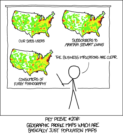
Comparing growth rates in crime versus population would likely yield a much better assessment of crime rates, but I haven’t found the right data (yet).
Ideally, I’d like to get current crime and total population data. By city would also be great. If I can find this data, I’ll put together another post.